Proving the Gaussian Integral

Sep 11, 2024
normal distribution statistics

Before proving the probability density function (PDF) of the normal distribution, it is essential to first understand the fundamental concept of the normal distribution itself, including its definition, properties, and mathematical form. A solid understanding of these basics will make the derivation process much clearer.

You can review the foundational material on normal distribution through the following reference: Learn about Normal Distribution Here

The Gaussian integral is defined as:

I = \int_{-\infty}^{\infty} e^{-x^2} \, dx

In this integral, (x) is only a dummy variable, so it can also be written as:

I = \int_{-\infty}^{\infty} e^{-y^2} \, dy

Suppose we multiply the two integrals:

I^2 = I \cdot I

I^2 = \left( \int_{-\infty}^{\infty} e^{-x^2} \, dx \right) \left( \int_{-\infty}^{\infty} e^{-y^2} \, dy \right)

= \int_{-\infty}^{\infty} \int_{-\infty}^{\infty} e^{-x^2} e^{-y^2} \, dx\,dy

= \int_{-\infty}^{\infty} \int_{-\infty}^{\infty} e^{-(x^2+y^2)} \, dx\,dy

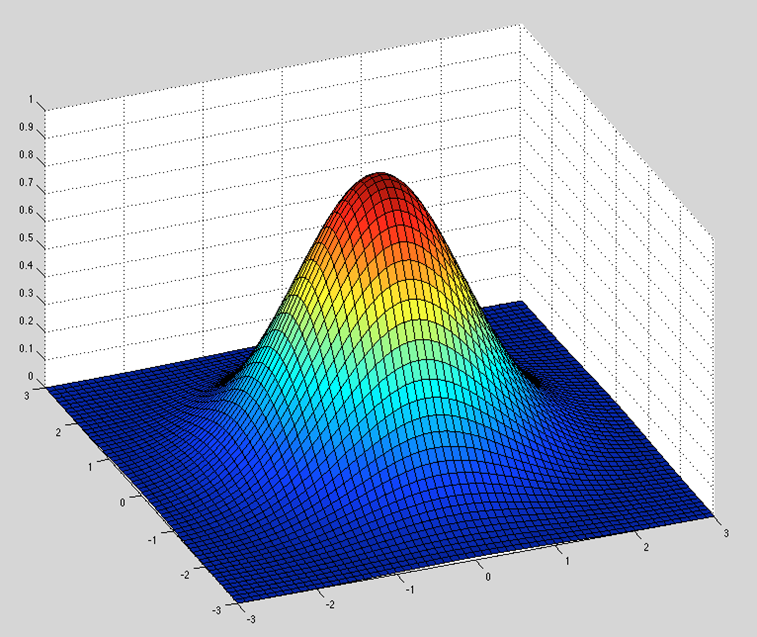
If the above function is visualized it will be Figure 1.

Gaussian Distribution Curve — Figure 1. Gaussian plot of the x and y integrals.

The two-variable function above resembles a single-variable Gaussian function, but with spherical symmetry. This means that any point located at the center (origin) has the same distance in every direction, making the function radially symmetric.

Because of this symmetry, the Gaussian integral can be more conveniently solved using the polar coordinate transformation. In polar coordinates, we only need:

The radial coordinate $r$ , ranging from $0$ to $\infty$ , to represent all possible distances from the origin.
The angular coordinate $\theta$ , ranging from $0$ to $2\pi$ , to cover the full circular rotation.

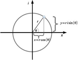
Using polar coordinates, the following relationships hold:

r^2 = x^2 + y^2

x = r \cos\theta

y = r \sin\theta

This transformation significantly simplifies the double integral and is the key step in deriving the Gaussian integral solution. Figure 2 illustrates the polar coordinate system and its corresponding variable relationships.

Gaussian Graph — Figure 2. Polar graph of r.

To transform the Cartesian differential element $dx\,dy$ into polar coordinates, we use the Jacobian determinant.

The Jacobian transformation is:

dx\,dy = \left| \frac{\partial(x,y)}{\partial(r,\theta)} \right| dr\,d\theta

= \begin{vmatrix} \frac{\partial x}{\partial r} & \frac{\partial x}{\partial \theta} \\ \frac{\partial y}{\partial r} & \frac{\partial y}{\partial \theta} \end{vmatrix} dr\,d\theta

For:

x = r\cos\theta

y = r\sin\theta

The Jacobian matrix becomes:

\begin{vmatrix} \cos\theta & -r\sin\theta \\ \sin\theta & r\cos\theta \end{vmatrix}

Its determinant is:

r(\cos^2\theta + \sin^2\theta) = r

Thus:

dx\,dy = r\,dr\,d\theta

Substituting into the Gaussian integral:

I^2 = \int_{-\infty}^{\infty} \int_{-\infty}^{\infty} e^{-(x^2+y^2)}\,dx\,dy

Transforming into polar coordinates:

= \int_0^{2\pi} \int_0^{\infty} e^{-r^2}\,r\,dr\,d\theta

Separating variables:

= \int_0^{2\pi} \left( \int_0^{\infty} r e^{-r^2}\,dr \right) d\theta

Evaluating the inner integral:

\int_0^{\infty} r e^{-r^2}\,dr = \left[ -\frac{1}{2}e^{-r^2} \right]_0^{\infty} = \frac{1}{2}

Therefore:

I^2 = \int_0^{2\pi} \frac{1}{2} \,d\theta

= \frac{1}{2}(2\pi)

I^2 = \pi

Thus:

I = \sqrt{\pi}

So the Gaussian integral is:

\int_{-\infty}^{\infty} e^{-x^2}\,dx = \sqrt{\pi}

Connection to Normal Distribution

Recall the probability density function (PDF) of the normal distribution:

f(x)=\frac{1}{\sigma\sqrt{2\pi}} e^{-\frac{(x-\mu)^2}{2\sigma^2}}

For:

$\mu = 0$
$\sigma = \frac{1}{\sqrt{2}}$

Substituting:

f(x)= \frac{1}{\sqrt{\pi}} e^{-x^2}

This proves that the Gaussian integral corresponds to the non-normalized form of the standard normal distribution curve, and its normalization constant is precisely derived from:

\int_{-\infty}^{\infty} e^{-x^2}\,dx = \sqrt{\pi}