Particle Swarm Optimization

Particle Swarm Optimization (PSO) is a stochastic population-based metaheuristic algorithm inspired by swarm intelligence (SI) [1]. Swarm intelligence is a field of artificial intelligence that studies how groups of simple agents (such as birds, fish, ants, or bees) can produce intelligent collective behavior without centralized control or leadership.

PSO mimics the social behavior of bird flocks or fish schools when searching for food sources [2]. In such systems, cooperative behavior naturally emerges among individuals without the need for a central coordinator.

In the basic PSO model, a swarm consists of $N$ particles moving through a $D$-dimensional search space. Each particle $i$ represents a candidate solution and is denoted by its position vector:

Each particle has:

• A current position
• A velocity vector

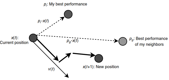
The optimization process in PSO relies on cooperation among particles, where each particle updates its position toward the global optimum by considering two key factors:

1. Personal Best Position ($pbest_i$):
   The best position previously found by particle $i$:

2. Global Best Position ($gbest$) or Local Best Position ($lbest$):
   The best position found by the entire swarm or a local neighborhood:

The difference between the current position and the best neighboring solution is represented by:

Through iterative position and velocity updates, particles collectively explore the search space and converge toward optimal or near-optimal solutions.

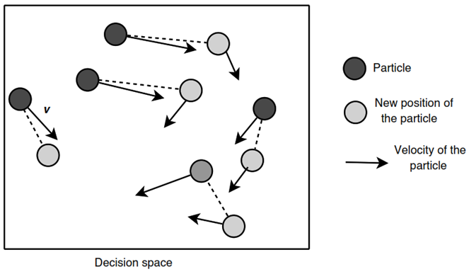
In each iteration, particles move from one position to another within the decision space. Unlike gradient-based optimization methods, PSO does not rely on gradient information during the search process [3].

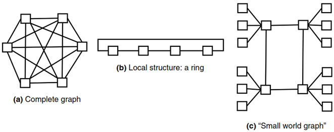
A key concept in PSO is the neighborhood structure, which determines the social influence among particles. The neighborhood defines how particles share information regarding the best solutions found so far.

Traditionally, there are two primary neighborhood models:

• Global Best (gbest):
  In the gbest model, the neighborhood of each particle includes the entire swarm population. Therefore, every particle is influenced by the best-performing particle in the whole swarm.

• Local Best (lbest):
  In the lbest model, particles interact only with a specific subset of neighboring particles based on a predefined topology. Thus, each particle is influenced only by the best solution found within its local neighborhood. If a particle has no connected neighbors, its neighborhood influence may be considered empty (e.g., $C_2 = 0$).

These neighborhood strategies significantly affect the balance between exploration and exploitation during the optimization process.

Basic Concept of Particle Swarm Optimization (PSO)

In PSO, each particle does not directly know the exact location of the optimal solution (food source). Instead, it relies on two primary sources of information:

1. Personal Experience (Personal Best / pbest)
2. Social Experience (Global Best / gbest or Local Best / lbest)

This mechanism is inspired by the natural dynamics of bird flocks and fish schools.

Biological Inspiration

In real-world swarm behavior, birds or fish do not possess precise knowledge of food locations. Instead, they depend on local sensory information and social interactions within the group.

The biological process can be summarized as follows:

1. Local Sensing

When an individual detects signs of food—such as scent, movement, or visual cues—it changes its speed and direction. Nearby individuals observe and respond to this movement.

2. Social Following

There is no permanent leader within the swarm. Therefore, when one individual suddenly moves rapidly toward a particular direction, others interpret this as useful information and instinctively follow, increasing their collective chance of finding food.

3. Information Propagation

When one individual discovers food or detects a promising region:

• It moves toward that area (personal best)
• Its movement influences nearby individuals
• The behavioral information spreads throughout the swarm
• Other members adjust their movement accordingly (global best)

This natural collective intelligence forms the foundation of PSO, where particles iteratively update their velocities and positions based on both personal memory and social cooperation to search for the optimal solution.

Working Mechanism of Particle Swarm Optimization (PSO)

The PSO algorithm searches for optimal solutions through iterative population-based exploration [3]. The general process is as follows:

1. Population Initialization

A swarm of particles is initialized with random positions and velocities within the search space.

2. Fitness Evaluation

Each particle is evaluated using an objective (fitness) function:

This function is problem-dependent and designed according to the optimization objective.

The evaluation determines:

• Personal best position ($pbest_i$)
• Global best position ($gbest$) or local best ($lbest$)

3. Velocity Update

The original velocity update formula is:

Where:

• $v_i(t-1)$ = previous velocity (momentum)
• $\rho_1, \rho_2$ = random numbers from $U(0,1)$
• $C_1$ = cognitive learning factor (self-learning strength)
• $C_2$ = social learning factor (neighbor-following strength)
• $(p_i - x_i)$ = direction toward personal best
• $(p_g - x_i)$ = direction toward social/global best

Inertia Weight Version

A more commonly used modern formula introduces inertia weight $w$ [4]:

The inertia weight $w$ controls the influence of previous velocity:

• Large $w$ → stronger global exploration
• Small $w$ → stronger local exploitation

Thus, inertia weight balances:

• Exploration: broad search
• Exploitation: intensive local refinement

4. Position Update

After updating velocity, the particle position is updated:

5. Best Solution Update

Each particle updates its personal best:

The global best is also updated:

6. Termination

The iterative process stops when stopping criteria are met, such as:

• Maximum iterations reached
• Desired fitness achieved
• Convergence threshold satisfied

Through repeated updates of velocity, position, and best solutions, PSO efficiently converges toward optimal or near-optimal solutions.

References

[1] Kennedy, J., Eberhart, R. C., & Shi, Y. (2001). Swarm Intelligence. Evolutionary Computation Series. Elsevier Science. https://doi.org/10.1016/B978-1-55860-595-4.X5000-1
[2] Kennedy, J., & Eberhart, R. (1995). Particle swarm optimization. In Proceedings of ICNN’95 - International Conference on Neural Networks (pp. 1942–1948). IEEE. https://doi.org/10.1109/ICNN.1995.488968
[3] Talbi, E. G. (2009). Metaheuristics: From Design to Implementation. Wiley Series on Parallel and Distributed Computing. Wiley.
[4] Shi, Y., & Eberhart, R. (1998). A modified particle swarm optimizer. In 1998 IEEE International Conference on Evolutionary Computation Proceedings (pp. 69–73). IEEE. https://doi.org/10.1109/ICEC.1998.699146
[5] Chin, R. (2025). Particle Swarm Optimization. Retrieved November 19, 2025.
[6] Wikipedia. (2025). Particle Swarm Optimization. Retrieved November 19, 2025.